“How many respondents do I need?” is one of the first questions in any action research, and the most common answer in Philippine schools is Slovin’s formula. This guide explains what the Department of Education’s (DepEd) Action Research Toolkit says about sampling and sample size, what Slovin’s formula really does and when it fits, and how to tell whether a class-sized study can detect the effect it is looking for. It uses real DepEd data: the number of public schools in each schools division, and the number of learners a typical school assesses in the Comprehensive Rapid Literacy Assessment (CRLA).
It is written for teachers planning action research, for school heads and division research staff who review proposals, and for graduate students planning surveys of schools.
Key points
- The toolkit’s rules of thumb. At least 30 per group for experiments and causal-comparative studies, at least 50 for correlational studies, at least 100 for surveys, and as few as one for qualitative case studies, “preferably random” in each case.
- Action research usually samples whole classes. The toolkit notes that in action research “the sampling should be purposive and accessible”: the learners in the classroom with the problem.
- Slovin’s formula is for surveys only. It is the standard formula for estimating a percentage (with p = 0.5 and 95% confidence) with a correction for small populations. It is not meant for experiments, comparisons or correlations, which need a power analysis.
- Divisions are small populations. The median division has 57 public schools in the CRLA data and 78 in the classroom data. For a survey of a division’s schools to within ±5 points, Slovin’s formula asks for 50 of 57 schools, close to a census.
- Small groups can only detect large effects. With 30 learners per group, the toolkit’s minimum, a t-test has an 80% chance of detecting an effect of about 0.74 standard deviations. The median Grade 1 group in a school assessed 23 learners, which can detect about 0.84 with two groups or 0.61 with a pretest and posttest.
Population, accessible population and sample
The toolkit distinguishes three groups:
- the target population, “the entire group of individuals for which the intervention or treatment is envisioned to be useful”, such as all Grade 1 struggling readers in the division;
- the accessible population, the “subset of the target population” you can actually include, such as the Grade 1 learners in your school; and
- the sample, the subset of the accessible population you study. It “must be representative of the population from which it was selected to enable the application of the findings to the population”.
In most action research, the sample is the accessible population: the learners in your own class. That is fine for improving your own teaching, but it limits how far the results travel. Say so in the report.
Sampling methods
| Method | How it works | When it fits school research |
|---|---|---|
| Simple random | Every member has an equal chance, by lottery or random numbers | Choosing learners or schools for a survey from a complete list |
| Stratified random | Divide the population into groups (strata), then sample each in proportion | When subgroups differ, such as districts, grade levels, or boys and girls |
| Random cluster | Randomly choose whole groups, such as sections or schools | When learners are already grouped in classes; common in schools |
| Two-stage or multi-stage | Choose clusters at random, then individuals within them | Division studies: districts, then schools, then sections, then learners |
| Purposive | Choose members with a trait related to the study | Interventions for a specific group, such as Low Emerging readers |
| Systematic | Take every kth member of a list from a random start | Quick samples from an ordered list |
| Convenience | Whoever is available or willing | Pilot studies; results may not represent the population |
| Snowball | Participants refer others | Interviews with hard-to-find groups |
| Quota | Fill set numbers for each subgroup, not at random | When proportions matter but a random sample is not possible |
The toolkit classes systematic sampling as nonrandom, because once the start and interval are fixed, members no longer have an equal chance; many statistics textbooks treat systematic sampling with a random start as a probability method. Either way, describe exactly what you did.
Drawing a random sample in Excel
- List the population, one member per row, with a code (for example, school IDs or learner codes).
- In the next column, enter
=RAND()and copy it down. Each row gets a random number between 0 and 1. - Copy the random numbers and paste them as values, so they stop changing.
- Sort the list by the random-number column, and take the first n rows.
For a stratified sample, add a column for the stratum, such as the district, sort by stratum and then by the random number, and take the needed number from each stratum in proportion to its size. Keep the sorted file: it documents how the sample was drawn.
The toolkit’s suggested sample sizes
The toolkit suggests these minimums “to enable Action Researchers to apply statistical tools for the purpose of making general statements about an intervention or treatment”:
| Design | Suggested minimum |
|---|---|
| Experimental and causal-comparative | At least 30 per group, preferably random, “by the time the experiment finishes”, so start with more than 30 |
| Correlational | At least 50, preferably random |
| Survey | At least 100, preferably random |
| Qualitative | As few as 1, as in a case study; if more, chosen for maximum variation |
It adds a rule of thumb: “The smaller the population, the larger the sampling ratio should be.”
These are floors, not targets. What a sample can show depends on the size of the effect or the precision you need, which the next sections work out.
How many for a survey: Cochran’s and Slovin’s formulas
A survey estimates a percentage, such as the share of teachers who use the CRLA results to group learners, to within a margin of error. Cochran’s formula gives the sample size for a large population:
n₀ = z² × p × (1 − p) ÷ e²
where z is 1.96 for 95% confidence, p is the expected percentage (0.5 when unknown, which gives the largest sample), and e is the margin of error. For e = ±5 points, n₀ = 385; for ±10 points, 97. For a population of N members, the finite population correction lowers it:
n = n₀ ÷ (1 + (n₀ − 1) ÷ N)
Slovin’s formula, n = N ÷ (1 + N × e²), is the same calculation simplified: it assumes p = 0.5 and rounds z to 2, then applies a version of the correction. It appears in Taro Yamane’s 1967 statistics textbook and is widely attributed to Slovin. It gives nearly the same numbers as Cochran’s formula:
| Schools in the population | Margin of error | Cochran (p = 0.5, 95%) | Slovin |
|---|---|---|---|
| 57 | ±5 points | 50 | 50 |
| 57 | ±10 points | 37 | 37 |
| 78 | ±5 points | 65 | 66 |
| 78 | ±10 points | 44 | 44 |
| 300 | ±5 points | 169 | 172 |
| 300 | ±10 points | 73 | 75 |
| 1,000 | ±5 points | 278 | 286 |
| 1,000 | ±10 points | 88 | 91 |
Three things follow. First, Slovin’s formula is fine for what it was made for: estimating a percentage in a survey. Second, for small populations, such as the schools in a division, it asks for nearly everyone; with 57 schools, surveying all of them is simpler and removes sampling error altogether. Third, it says nothing about experiments, comparisons between groups or correlations, where the question is not “how precise is my percentage?” but “can my study detect the difference I am looking for?” For those, use a power analysis.
How many divisions and schools: the real numbers
DepEd’s schools divisions vary enormously in size. In the end-of-year CRLA for SY 2025-26, the 232 divisions have a median of 57 public schools, from 9 to 1,111, and 51 divisions have fewer than 30. In the 2023 classroom shortage data, the 229 divisions have a median of 78 schools, from 13 to 1,270.
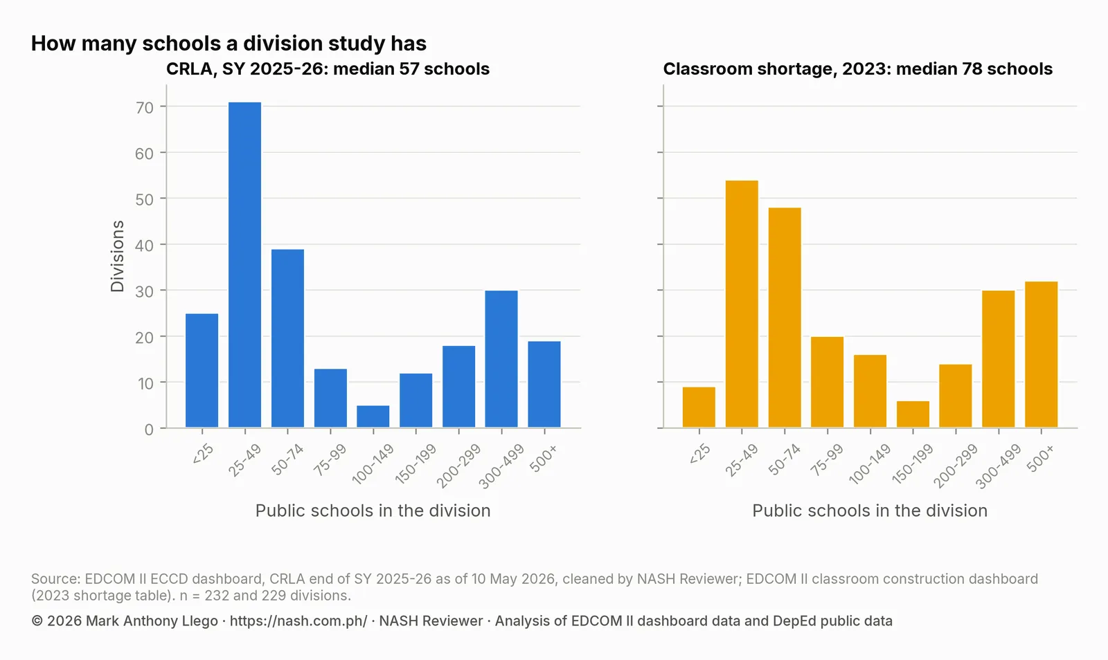
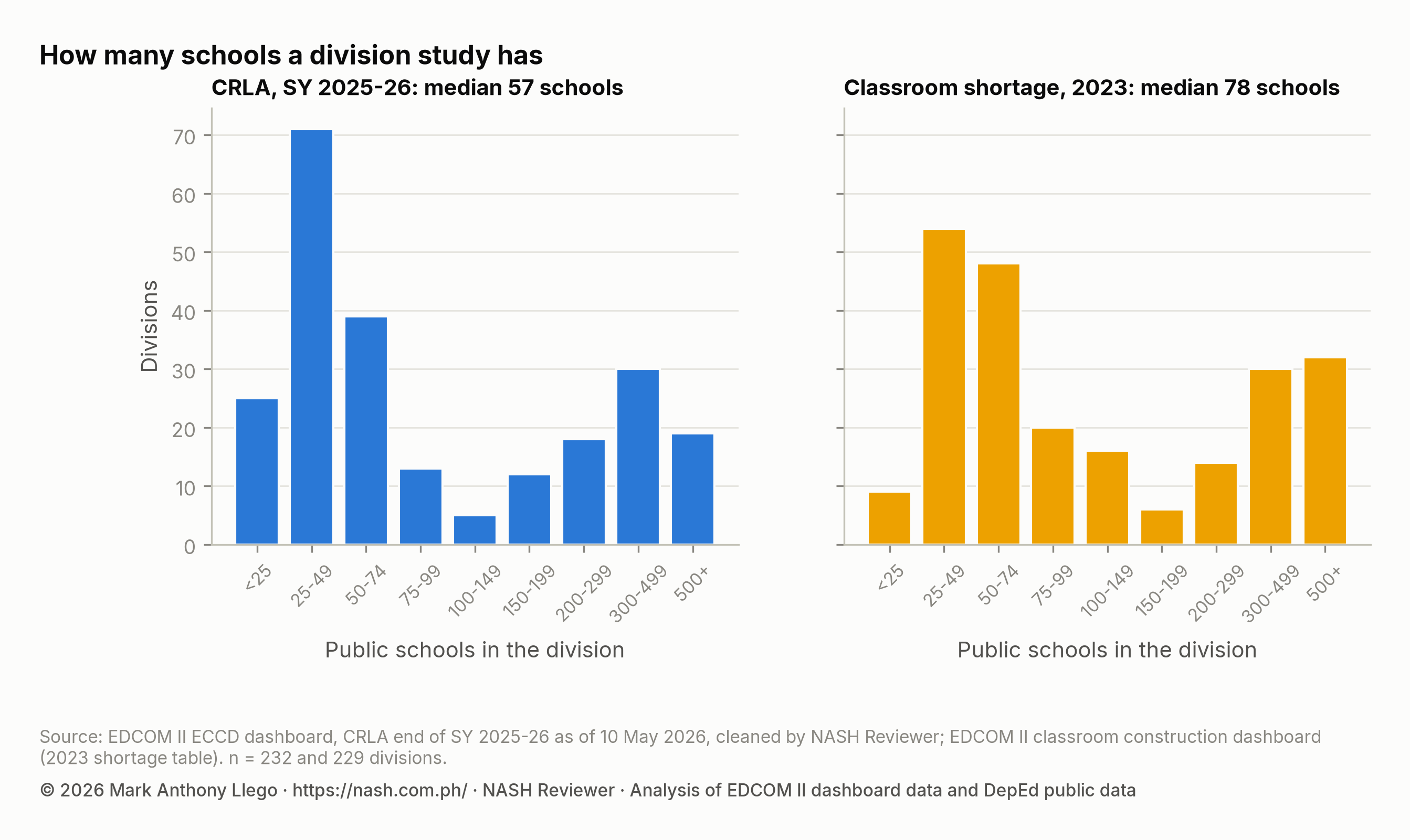
For a division study that uses schools as the unit, such as comparing schools with and without a feature, the whole division is often fewer schools than a survey formula would ask for. Study all of them, and remember that a study of 57 schools has the statistical power of 57 cases, however many learners they enroll.
Schools themselves are small samples of learners. The median school assessed 71 learners in the CRLA, and the median Grade 1 group 23; 6,173 schools assessed fewer than 30 learners. A school’s share of struggling readers can swing widely by chance: How to Read a School’s CRLA Results Fairly shows that the median 95% interval is 17 percentage points wide in schools with fewer than 30 learners, against 4 points in the largest.
How many for an experiment: power
An action research that compares a class before and after, or an intervention group with a comparison group, needs enough learners to detect the effect it expects. Four things decide the sample size:
- The effect size, the difference you expect divided by the standard deviation (Cohen’s d). Cohen’s rough guide calls 0.2 small, 0.5 medium and 0.8 large.
- The significance level, usually alpha = 0.05, two-sided.
- The power, the chance of detecting a real effect of that size, usually set at 80%.
- The design: two groups, or one group measured twice. A paired design needs fewer learners because each learner serves as their own comparison.
| Effect size (Cohen’s d) | Learners per group, two groups | Learners in all, two groups | Learners, one group measured twice |
|---|---|---|---|
| Small (0.2) | 394 | 788 | 199 |
| Medium (0.5) | 64 | 128 | 34 |
| Large (0.8) | 26 | 52 | 15 |
Turned around, a fixed number of learners can only detect effects above a certain size:
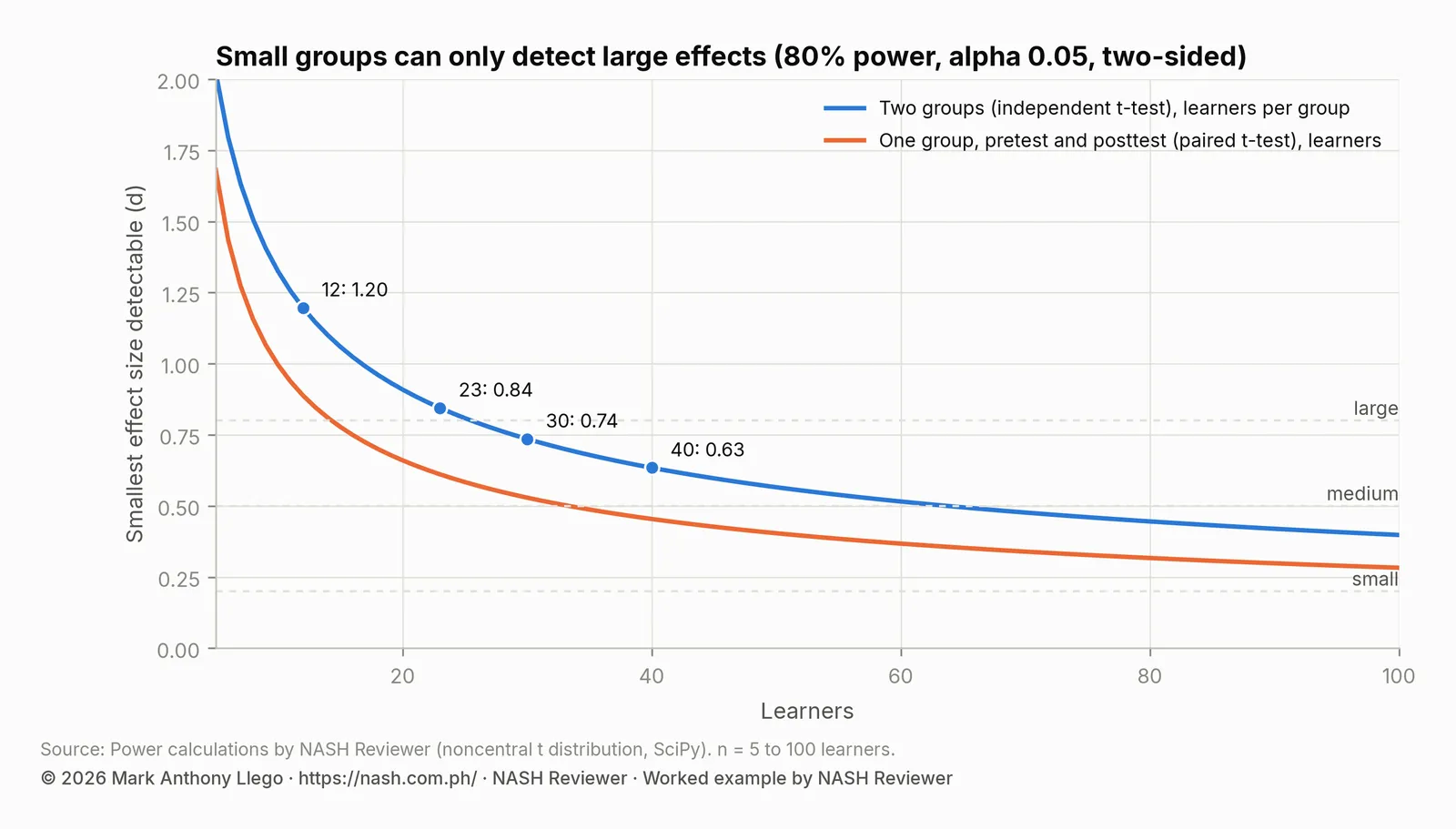
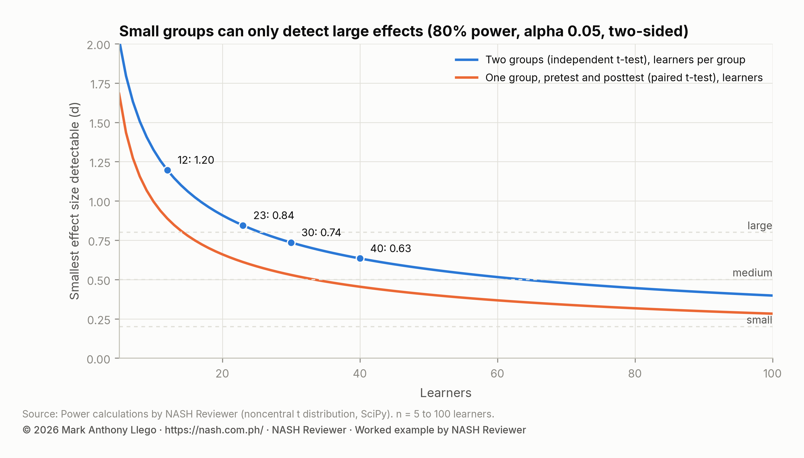
- With 12 learners per group, the size of the toolkit’s t-test exercise, only effects of about 1.20 standard deviations or more are reliably detected (0.89 in a paired design).
- With 23 learners, the median Grade 1 group in the CRLA, about 0.84 for two groups or 0.61 for a pretest and posttest.
- With 30 per group, the toolkit’s minimum, about 0.74 (0.53 paired).
- With 40 per group, a large class, about 0.63 (0.45 paired).
Many classroom interventions have effects well below 0.5. A small study that finds “no significant difference” has often simply been too small to see the effect; it is not evidence that the intervention does not work. And a small study that does find a significant effect may have overestimated it.
A paired design has one more catch: its effect size (dz) depends on how closely the pretest and posttest scores correlate. And a one-group design detects ordinary growth as readily as an intervention effect; Pretest-Posttest Design and Regression to the Mean explains why a comparison group is still needed.
How many for a correlation
The toolkit suggests at least 50 for correlational studies. The reason is precision: with 30 pairs, a correlation must be at least 0.36 to reach p < 0.05 (two-sided); with 50, 0.28; with 100, 0.20. Weak but real relationships, such as most links between school inputs and learning outcomes, need large samples to show.
Learners in classes: why clusters matter
Learners in the same class share a teacher, a room and a timetable, so their scores are more alike than those of learners chosen at random. Thirty learners from one section carry less independent information than thirty learners from thirty sections. Two practical rules follow:
- When the intervention is given to whole classes, count classes. An experiment with one intervention section and one comparison section is, in effect, a comparison of two classes; any difference between the teachers or the class schedules is mixed into the result. Use several sections per group when you can, or have the same teacher teach both.
- When sampling across schools, sample the schools first. The toolkit’s multi-stage sampling (districts, then schools, then sections, then learners) does this, and the analysis should account for it, for example by comparing school averages.
What to do with a small class
- Use a paired design and a comparison group together. Measure every learner before and after, and compare the gains of two groups.
- Combine classes. Teachers of parallel sections in a Learning Action Cell can run the same study in several classes, which raises the numbers and spreads out teacher effects.
- Measure well. A longer, more reliable test reduces the noise that small samples cannot average away.
- Report effect sizes and intervals. Say how big the change was and how uncertain the estimate is, not only whether p was below 0.05.
- Add qualitative evidence. Observations and interviews can show how and for whom an intervention worked, which numbers from 20 learners cannot.
- State the limits. A study of one class tells you about that class; say so, and present the results as a basis for a larger study.
Common mistakes
- Using Slovin’s formula for an experiment. It sizes a survey estimate, not a comparison of groups.
- Sampling from a small population. With 57 schools, study all 57.
- Treating “no significant difference” as “no effect”. A small study may lack the power to see a real effect.
- Counting learners when classes were assigned. Two sections are two clusters, not 80 independent learners.
- Losing learners without saying so. The toolkit’s 30 per group means 30 at the end; start with more, and report attrition.
- Calling a convenience sample random. Describe how participants were actually chosen.
Frequently asked questions
What is Slovin’s formula?
n = N ÷ (1 + N × e²), where N is the population size and e is the margin of error. It gives the sample size for estimating a percentage in a survey with about 95% confidence, assuming the true percentage is near 50%. It is a simplified form of Cochran’s formula with a correction for small populations, and it is not designed for experiments or comparisons between groups.
How many respondents do I need for an action research?
It depends on the design. DepEd’s Action Research Toolkit suggests at least 30 per group for experiments, 50 for correlational studies and 100 for surveys. For an experiment, a power analysis is better: detecting a medium effect (0.5 standard deviations) with 80% power needs about 64 learners per group, or 34 learners measured twice.
Is it acceptable to use my whole class as the sample?
Yes. The toolkit notes that in action research “the sampling should be purposive and accessible”: the learners in the class with the problem. Describe the class, explain that the results apply to it, and add a comparison group if you want to judge the intervention’s effect.
How do I choose a random sample in Excel?
List the population with codes, add =RAND() in the next column, paste the results as values, sort by that column and take the first n rows. For a stratified sample, sort by stratum first and take the needed number from each.
Why does my action research show no significant difference?
Often because the sample was too small to detect the effect. With 23 learners per group, only effects of about 0.84 standard deviations or more are reliably detected. Report the effect size and its interval, and treat the study as a pilot for a larger one rather than as proof that the intervention does not work.
More on DepEd research
- Start here: DepEd Action Research Guide: From Topic to Report
- Survey Research With Google Forms for Action Research
- Paired and Independent t-Test in Excel for Action Research
- Pretest-Posttest Design and Regression to the Mean
- DepEd Action Research Proposal Format, With a Sample
- BERF: How to Get DepEd Action Research Funded
- Topics with data: Action Research and Thesis Topics on Classroom Shortage, Action Research and Thesis Topics on Reading (CRLA)
- Related: How to Read DepEd Data: A Guide for Aspiring School Heads
Sources
- Department of Education and the Basic Education Sector Transformation (BEST) Program. (2019). Action Research Toolkit: Teacher’s Guide, sections 3.1 (experimental designs) and 4.1 (sampling methods), with support from the Australian Government.
- Cochran, W. G. (1977). Sampling techniques (third edition). John Wiley & Sons.
- Yamane, T. (1967). Statistics: An introductory analysis (second edition). Harper and Row.
- Cohen, J. (1988). Statistical power analysis for the behavioral sciences (second edition). Lawrence Erlbaum Associates.
- Division sizes and CRLA school sizes: the EDCOM II early-childhood dashboard data and the EDCOM II classroom data, cleaned by NASH Reviewer.
- Power calculations: the noncentral t distribution in Python with SciPy, 80% power and alpha 0.05, two-sided.
Analysis and charts by Mark Anthony Llego for NASH Reviewer. NASH Reviewer is not affiliated with DepEd or EDCOM II.