A t-test compares two means. When an action research compares three or more groups, such as three sections taught with different strategies or schools of three sizes, the test is the analysis of variance (ANOVA). The Department of Education’s (DepEd) Action Research Toolkit lists the one-way ANOVA among the “other useful inferential statistics”, “for comparing three or more means” (section 5.3), but does not show how to run it. Here it is in Excel, with the toolkit’s own posttest data and with real reading results from DepEd’s Comprehensive Rapid Literacy Assessment (CRLA).
It is written for teachers and school heads analyzing action research data, and for graduate students. Few classroom studies need ANOVA; when one does, this is the procedure.
Key points
- Use ANOVA for three or more group means. For two groups, use a t-test. Running several t-tests instead raises the chance of a false positive: with four groups and six t-tests at 0.05, it is up to 26%.
- One menu in Excel. Data > Data Analysis > Anova: Single Factor gives the F statistic, its p-value and the critical F.
- A significant F says only that some means differ. A post hoc test tells you which; Excel has none built in, so use t-tests with a Bonferroni correction, or a free program for Tukey’s test.
- Report the effect size. Eta squared (η²) = between-groups sum of squares ÷ total sum of squares. In the toolkit’s data it is 0.76; for CRLA results by school size nationally it is 0.002, significant only because there are 35,281 schools.
- Check the assumptions: independent cases, roughly normal scores in each group, and similar spreads.
When to use one-way ANOVA
| Your question | Test |
|---|---|
| Do two groups differ in mean score? | t-test |
| Do three or more groups differ in mean score? | One-way ANOVA |
| Do two factors, such as strategy and gender, affect a score, and do they interact? | Two-way ANOVA |
| Do groups differ in the share with some outcome (counts)? | Chi-square test |
| Scores are ranks or badly skewed, with three or more groups | Kruskal-Wallis test |
Hypotheses. Null: all the group means are equal. Research: at least one mean differs from the others.
Why not several t-tests? Each test at alpha = 0.05 carries a 5% chance of a false positive. Four groups make six pairs, and the chance that at least one of six independent tests is falsely significant is 1 − 0.95⁶ = 26%. ANOVA tests all the groups at once at 5%.
One-way ANOVA in Excel, step by step
The example is the toolkit’s own data (Table 5.1.1 in section 5.1): posttest scores on a 10-item language test after a six-month intensive English program, for girls and boys in an experimental and a control group, 10 learners in each.
Step 1. Load the Analysis ToolPak once: File > Options > Add-ins > Manage Excel Add-ins > Go > tick Analysis ToolPak. (Microsoft’s instructions.)
Step 2. Enter the data with one column per group and the group names in row 1:
| Experimental girls | Experimental boys | Control girls | Control boys |
|---|---|---|---|
| 6 | 8 | 4 | 6 |
| 5 | 7 | 5 | 5 |
| 7 | 9 | 4 | 4 |
| 6 | 7 | 3 | 5 |
| 5 | 10 | 4 | 6 |
| 6 | 8 | 5 | 5 |
| 5 | 9 | 4 | 4 |
| 7 | 7 | 3 | 5 |
| 6 | 7 | 5 | 6 |
| 7 | 8 | 3 | 4 |
Step 3. Run the test. Data > Data Analysis > Anova: Single Factor. Input range A1:D11; Grouped by Columns; tick Labels in first row; Alpha 0.05; choose an output cell. Excel returns two tables.
SUMMARY:
| Groups | Count | Sum | Average | Variance |
|---|---|---|---|---|
| Experimental girls | 10 | 60 | 6.0 | 0.667 |
| Experimental boys | 10 | 80 | 8.0 | 1.111 |
| Control girls | 10 | 40 | 4.0 | 0.667 |
| Control boys | 10 | 50 | 5.0 | 0.667 |
ANOVA:
| Source of variation | SS | df | MS | F | P-value | F crit |
|---|---|---|---|---|---|---|
| Between groups | 87.5 | 3 | 29.167 | 37.50 | 3.59E-11 | 2.866 |
| Within groups | 28.0 | 36 | 0.778 | |||
| Total | 115.5 | 39 |
Step 4. Read the result. F = 37.50 is far above the critical value of 2.866, and the p-value, 3.59E-11, means 0.0000000000359. Reject the null hypothesis: the four group means are not all equal.
What the table means. The total variation in scores (SS total = 115.5) splits into variation between the group means (87.5) and variation within the groups (28.0). Each is divided by its degrees of freedom to give a mean square (MS). F is the ratio of the two mean squares, 29.167 ÷ 0.778: here the differences between groups are 37.5 times larger than the variation you would expect from chance.
Step 5. Measure the size of the effect. η² = SS between ÷ SS total = 87.5 ÷ 115.5 = 0.76: group membership accounts for 76% of the variation in scores. A common rough guide calls 0.01 small, 0.06 medium and 0.14 large.
Without the ToolPak
The same numbers with formulas, for scores in A2:D11:
- SS total:
=DEVSQ(A2:D11)→ 115.5 - SS within:
=DEVSQ(A2:A11)+DEVSQ(B2:B11)+DEVSQ(C2:C11)+DEVSQ(D2:D11)→ 28.0 - SS between: SS total − SS within → 87.5
- F:
=(87.5/3)/(28/36)→ 37.50 - p-value:
=F.DIST.RT(37.5, 3, 36) - Critical F:
=F.INV.RT(0.05, 3, 36)→ 2.866
The degrees of freedom are k − 1 between groups (k = number of groups) and N − k within (N = number of learners).
Which groups differ: post hoc tests
The F test says that the means are not all equal, not which ones differ. A post hoc test compares each pair while keeping the overall error rate at 5%.
In Excel: t-tests with a Bonferroni correction. Run t-Test: Two-Sample Assuming Equal Variances for each pair, and multiply each p-value by the number of comparisons (six for four groups), capping at 1. It is simple but conservative.
Tukey’s HSD test is the usual choice; Excel does not have it, but free programs such as JASP and jamovi do. For the toolkit’s data:
| Comparison | Difference in means | Tukey HSD p | Tukey 95% interval | Bonferroni t-test p (× 6) |
|---|---|---|---|---|
| Experimental girls vs experimental boys | −2.0 | < 0.001 | −3.06 to −0.94 | < 0.001 |
| Experimental girls vs control girls | +2.0 | < 0.001 | +0.94 to +3.06 | < 0.001 |
| Experimental girls vs control boys | +1.0 | 0.071 | −0.06 to +2.06 | 0.081 |
| Experimental boys vs control girls | +4.0 | < 0.001 | +2.94 to +5.06 | < 0.001 |
| Experimental boys vs control boys | +3.0 | < 0.001 | +1.94 to +4.06 | < 0.001 |
| Control girls vs control boys | −1.0 | 0.071 | −2.06 to +0.06 | 0.081 |
Four of the six pairs differ significantly. The two one-point differences do not, by either method.
The better analysis: two-way ANOVA
The toolkit’s four groups are really two factors: the group (experimental or control) and gender. A two-way ANOVA tests each factor and their interaction, that is, whether the program worked differently for girls and boys.
In Excel, arrange the data with the groups in two columns (experimental, control) and the genders in rows: the 10 girls’ scores in rows 2 to 11 and the 10 boys’ in rows 12 to 21, with labels in row 1 and column A. Then Data > Data Analysis > Anova: Two-Factor With Replication, with Rows per sample = 10. Excel calls the row factor “Sample” (here, gender) and the column factor “Columns” (here, the group).
| Source | SS | df | MS | F | p |
|---|---|---|---|---|---|
| Group (experimental or control) | 62.5 | 1 | 62.5 | 80.36 | p < 0.001 |
| Gender | 22.5 | 1 | 22.5 | 28.93 | p < 0.001 |
| Interaction | 2.5 | 1 | 2.5 | 3.21 | p = 0.081 |
| Within | 28.0 | 36 | 0.778 |
The experimental group scored 2.5 points higher on average (7.0 against 4.5), and boys 1.5 points higher than girls in both groups. The interaction is not significant: the program’s advantage was 2 points for girls and 3 for boys, a difference that could be chance with 10 learners per cell. This is the analysis that matches the toolkit’s design, and it answers the question a teacher would ask: did the program work, and for whom?
A real example: struggling readers by school size
Does the share of struggling readers differ between small, medium and large elementary schools? The CRLA results at the end of School Year (SY) 2025-26 give each school’s share of Grade 1 to 3 learners at the two lowest reading levels; SY 2023-24 enrollment gives the school’s size.
Nationally, across 35,281 schools with at least 20 learners assessed, the mean shares of struggling readers are 10.6% in schools with 100 or fewer elementary learners, 11.0% in schools with 101 to 500, and 9.7% in schools with more than 500. The ANOVA is highly significant, F(2, 35,278) = 30.1, p < 0.001, but η² = 0.002: school size accounts for 0.2% of the differences between schools. With 35,000 schools, even trivial differences are significant.
In one division, the Schools Division of Isabela City in Region IX, with 51 such schools:
| Elementary learners (SY 2023-24) | Schools | Mean struggling (%) | SD | Variance | National mean (%) |
|---|---|---|---|---|---|
| 100 or fewer | 9 | 20.6 | 16.1 | 258.8 | 10.6 |
| 101 to 500 | 32 | 21.7 | 16.7 | 279.7 | 11.0 |
| Over 500 | 10 | 21.0 | 14.5 | 210.0 | 9.7 |
F(2, 48) = 0.02, p = 0.981, below the critical value of 3.191; η² = 0.001. School size makes no difference here: the three means are within about a point of each other, while schools within each size group differ by 40 points or more (from 0% to 44% among the smallest schools, and from 2% to 78% among the middle-sized ones).
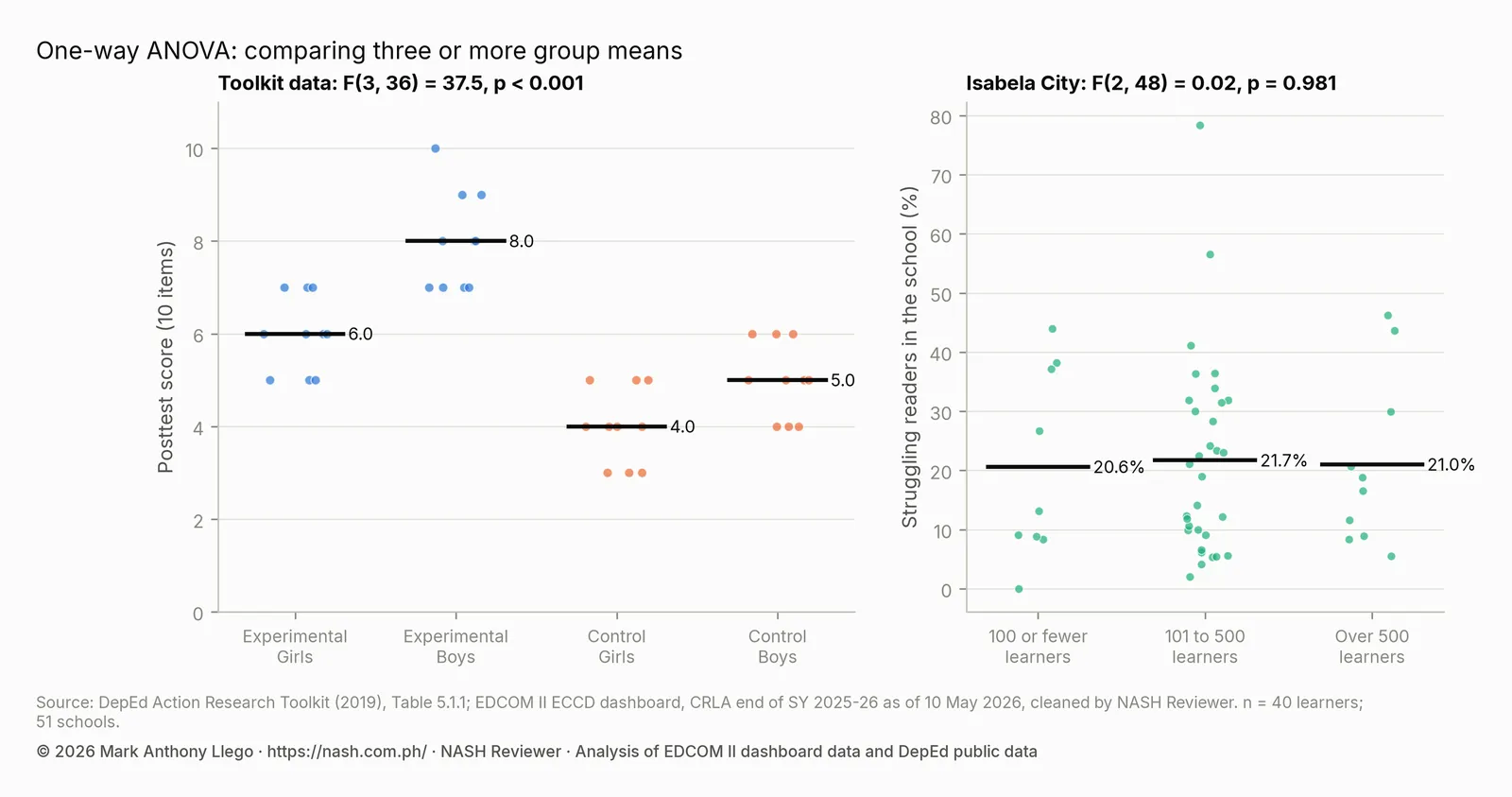
The two panels show what F measures. On the left, the group means are far apart compared with the spread inside each group; on the right, the spread inside each group dwarfs the differences between means. Among the 8 divisions with 40 to 90 eligible schools and at least 8 in each size group, Isabela City’s η² is the closest to the national value.
Assumptions to check
- Independent cases. Each learner or school appears in one group only. Repeated measurements of the same learners, such as a pretest, midtest and posttest, need a repeated-measures ANOVA instead.
- Roughly normal scores in each group. ANOVA tolerates moderate departures, especially with similar group sizes. For ranks, ratings on a few points, or badly skewed scores, use the Kruskal-Wallis test.
- Similar spreads. A rough check: the largest group variance should be no more than about four times the smallest (here 1.111 and 0.667 in the toolkit’s data). A formal check is Levene’s test, which Excel can do in its median-based form: replace every score by its distance from its group’s median (
=ABS(A2-MEDIAN(A$2:A$11))) and run Anova: Single Factor on those distances. For the toolkit’s data, p = 0.801; in Isabela City, p = 0.859, so equal spreads are reasonable. If spreads differ a lot, use Welch’s ANOVA (in JASP or jamovi); in Isabela City it gives the same verdict, F(2, 17.3) = 0.02, p = 0.982.
How to report a one-way ANOVA
Posttest scores differed among the four groups, F(3, 36) = 37.50, p < 0.001, η² = 0.76. Tukey’s test showed that the experimental boys (M = 8.0) scored higher than every other group, and the experimental girls (M = 6.0) higher than the control girls (M = 4.0).
Give the group means (and standard deviations) in a table, F with both degrees of freedom, the p-value, η², and the post hoc results.
Common mistakes
- Running t-tests on every pair instead of ANOVA, without any correction.
- Stopping at “significant”. Say which groups differ, by how much, and how large the effect is.
- Treating a non-significant F as proof of no difference in a small study. In Isabela City the evidence is strong because the means are nearly identical, not because p is large.
- Using ANOVA for counts or percentages of learners. For “how many passed” in each group, use the chi-square test.
- Ignoring the design. Two factors call for a two-way ANOVA, and the same learners measured three times call for a repeated-measures ANOVA.
Frequently asked questions
How do you do a one-way ANOVA in Excel?
Load the Analysis ToolPak, enter each group’s scores in its own column with a label in the first row, then choose Data > Data Analysis > Anova: Single Factor, select the data, tick Labels in first row and set alpha to 0.05. Compare F with F crit, or the p-value with 0.05.
What is F crit in Excel’s ANOVA output?
The critical value of F at your alpha, =F.INV.RT(0.05, df between, df within). If F is larger than F crit, the result is significant; this is the same decision as p < 0.05.
When should I use ANOVA instead of a t-test?
When you compare the means of three or more groups. A t-test compares two; running several t-tests instead inflates the chance of a false positive.
Does Excel have a post hoc test for ANOVA?
No. You can run t-tests between pairs and multiply each p-value by the number of comparisons (the Bonferroni correction), or use a free program such as JASP or jamovi for Tukey’s HSD test.
What is eta squared?
The share of the total variation explained by group membership: the between-groups sum of squares divided by the total sum of squares. Roughly, 0.01 is small, 0.06 medium and 0.14 large.
More on DepEd research
- Start here: DepEd Action Research Guide: From Topic to Report
- Paired and Independent t-Test in Excel for Action Research
- Chi-Square Test in Excel for Action Research
- Pearson Correlation in Excel for Action Research
- Coding Guide and Data Cleaning in Excel for Action Research
- Action Research Sample Size: Slovin, Power and Sampling
- Related: CRLA End-of-Year Results SY 2025-26: All 18 Regions
Sources
- Department of Education and the Basic Education Sector Transformation (BEST) Program. (2019). Action Research Toolkit: Teacher’s Guide, sections 5.1 (preparing data for analysis; Table 5.1.1) and 5.3 (inferential statistics), with support from the Australian Government.
- CRLA results: EDCOM II dashboard data on the Comprehensive Rapid Literacy Assessment at the end of SY 2025-26, cleaned by NASH Reviewer; school sizes from DepEd’s SY 2023-24 school data.
- Microsoft. F.DIST.RT function, F.INV.RT function and DEVSQ function.
- Cohen, J. (1988). Statistical power analysis for the behavioral sciences (second edition). Lawrence Erlbaum Associates.
Analysis and chart by Mark Anthony Llego for NASH Reviewer. NASH Reviewer is not affiliated with DepEd.